Accessing results
Here is how to use the modules and scripts that allow you to conveniently access and visualize the results stored during analyses in the main output hdf5-file. We provide access tools for both Python and Matlab, but note that the access through Python provides more advanced features.
Python
Setting things up
Make sure that you are in the virtual environment for PEACOC (in case you decided to use one):
> workon peacoc
For me, the command line now looks like this:
(peacoc) weltgeischt@heulsuse:~/PEACOC_tutorial$
Navigate into the directory of PEACOC:
> cd PEACOC
I am now in (pwd for showing the current directory):
> pwd
/home/weltgeischt/PEACOC_tutorial/PEACOC
Start python or ipython:
> ipython
From within python, we first import some useful modules:
In [1]: import core.ea_management as eam
In [2]: import core.helpers as hf
In [3]: import matplotlib.pyplot as plt
In [4]: import numpy as np
Initialize recording object
There are two ways to initialize a recording object and thereby gain access to the data. First, you can initialize a recording object with its parameter file.
In [2]: paramfile = '/home/weltgeischt/PEACOC_tutorial/run_params/my_recording_params.yml'
In [6]: aRec = eam.Rec(init_ymlpath=paramfile)
Alternatively, you could initialize it directly with the results file results file. If you want to plot colorful bursts, this option also requires you to give the path to the SOM.
In [3]: datapath = '/home/weltgeischt/PEACOC_tutorial/my_results/data/my_recording/my_recording__blipSpy.h5'
In [8]: sompath = '/home/weltgeischt/PEACOC_tutorial/PEACOC/config/som.h5'
In [9]: aRec = eam.Rec(init_datapath=datapath,sompath=sompath)
Note
If you dislike objects and want to extract the data directly from the hdf5 file, you are allowed to skip ahead.
Visualize EA sequences
Now let’s plot the LFP and the EA we detected:
In [4]: aRec.plot(['raw','artifacts','spikes','singlets','bursts'],legendOn=True)
In [11]: plt.show()
In the resulting plot you see the LFP trace (bottom), all spikes detected (middle, red ticks), and the sequence of bursts (top colored according to category) and solitary spikes (black ticks). The part of the LFP that we annotated as artifact was disregarded for analyses and is shown in a yellow shade:
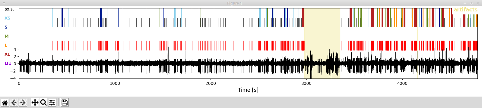
In this representation you see t-shirt size categorization which allow for a finer distinction that the one given in the paper_. XS and S bursts correspond to low-load bursts, M bursts are medium-load bursts, and XL and L bursts correspond to high-load bursts. In this representation bursts with a spike load index = 1 (LI1) are marked in purple (technically these are also XL bursts).
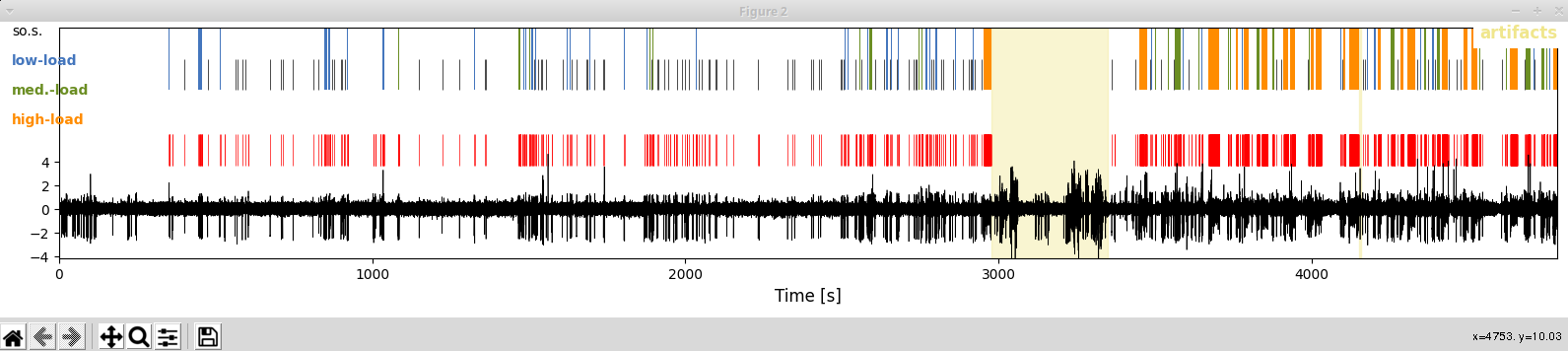
If you prefer the more compact, load-based categorizations (as in the papers) you can switch the naming scheme and coloring by executing:
In [5]: aRec.loadify_bursts()
As you can see when plotting now, colors and cluster identity are now given in the load scheme:
In [6]: aRec.plot(['raw','artifacts','spikes','singlets','bursts'],legendOn=True,loadlegend=True)
In [14]: plt.show()
Accessing the results (examples)
The recording object provides a convenient access to everything that was analyzed:
In [7]: aRec.dur# duration of whole recording
Out[7]: 4784.398

In [8]: aRec.offset #the time we excluded at the beginning ot the recording
Out[8]: 300

In [9]: aRec.artifactTimes #start and stop times of annoted artifacts
Out[9]:
array([[2978.61, 3348.16],
       [4153.07, 4157.07]])

In [10]: aRec.durAnalyzed# duration - offset - artifact times
Out[10]: 4110.848
You can directy extract the spiketimes and e.g. calculate the overall spike rate from it:
In [11]: aRec.spiketimes #timepoints of spikes detected
Out[11]: array([ 350.472,  352.368,  353.184, ..., 4783.702, 4784.058, 4784.198])

In [12]: spikerate = len(aRec.spiketimes)/aRec.durAnalyzed

In [13]: print (spikerate,'spikes/second')
0.4208377444264541 spikes/second
Our recording object contains a list of burst objects, that is the bursts that happend during the recording:
In [14]: aRec.bursts #list of burst objects
Out[14]:
[<core.ea_management.Burst at 0x7f79bd806c88>,
 <core.ea_management.Burst at 0x7f79b7cd2e48>,
 <core.ea_management.Burst at 0x7f79b7cd2b70>,
    .......................................
 <core.ea_management.Burst at 0x7f79b7cf16d8>]
Each burst object has a start and stop point in time (.start,`.stop`), a duration (.dur), a category (.cname), a color (.color, useful for plotting), a listing of its constituent spikes (.spiketimes), a spike load index (.si) and a few other properties.
In [15]: B = aRec.bursts[10]# for example lets pick burst number 10 and name it

In [16]: B.start
Out[16]: 919.578

In [17]: B.stop
Out[17]: 923.682

In [18]: B.roi #start and stop time
Out[18]: [919.578, 923.682]

In [19]: B.dur
Out[19]: 4.104000000000042

In [20]: B.cname
Out[20]: 'low-load'

In [21]: B.color
Out[21]: '#4476bd'

In [22]: B.spiketimes
Out[22]: array([919.578, 921.264, 923.258, 923.682])

In [23]: B.si #None because not classified on the SOM (<5 spikes), so lets pick a different example ...

In [24]: aRec.bursts[33].si
Out[24]: 0.17557326391422834
You can collect burst objects of a certain type and perform computations on them. Let’s e.g. collect high-load bursts and calculate their rate:
In [25]: hl_bursts = [B for B in aRec.bursts if B.cname=='high-load'] #list of burst objects
In [34]: N_hl = len(hl_bursts) #number of high-load bursts
In [35]: rate_hl = N_hl/aRec.durAnalyzed
In [36]: print ('High-load rate (/min): ', rate_hl*60.)#*60 to get /min
High-load rate (/min):  0.2919105741686387
Similarly we can also calculate the absolute time spent in high-load bursts and the fraction of time spent in high-load bursts:
In [26]: dur_hl = np.sum([B.dur for B in hl_bursts])

In [27]: print ('Total hl-duration (min): ', dur_hl/60.)#/ 60 to get min
Total hl-duration (min):  5.909600000000008

In [28]: print ('Relative time in high-loads: ', dur_hl/aRec.durAnalyzed)#/ 60 to get min
Relative time in high-loads:  0.08625373645534948
You can also address EA-free snippets as objects, in a way very similar to bursts:
In [29]: aRec.freesnips #list of EA-free snippet objects in the recording
Out[29]:
[<core.ea_management.Period at 0x7f79b410cda0>,
 <core.ea_management.Period at 0x7f79b410cdd8>,
 <core.ea_management.Period at 0x7f79b410ccc0>,
    .......................................
 <core.ea_management.Period at 0x7f79b4114c18>]

In [30]: aFree = aRec.freesnips[10] #10th EA-free snippet

In [31]: aFree.roi #start and stop time
Out[31]: [586.5360000000001, 593.752]

In [32]: aFree.dur #duration
Out[32]: 7.2159999999998945
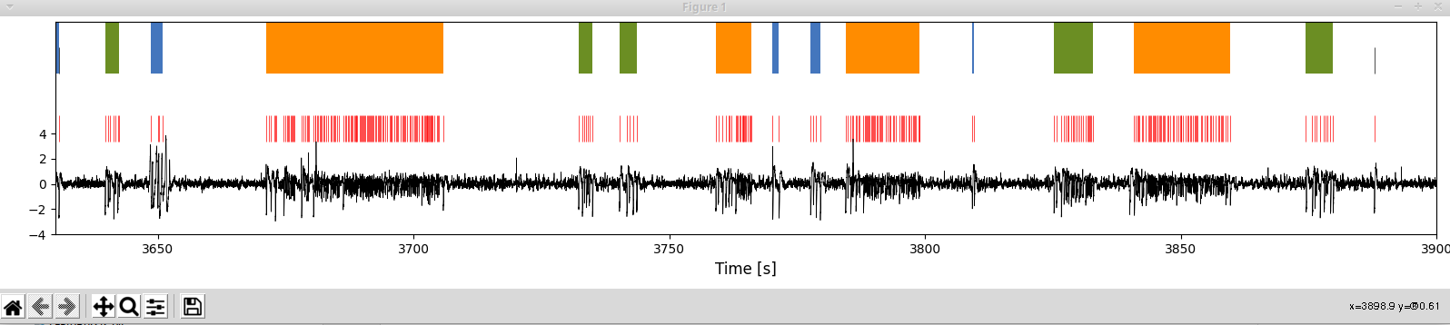
If you want to concentrate your analysis on a particular cutout of data you can do so too. The cutout can then be analysed and visualized in the same way as a the whole recording
In [33]: cutRec = eam.EAPeriod(3630.,3900.,parentobj=aRec) #cut out from recording object

In [34]: cutRec.bursts[10].dur #duration of the 10th burst in the cutout
Out[34]: 0.43039182282791444

In [35]: print ('Cutout spikerate: ',len(cutRec.spiketimes)/cutRec.dur,'spikes/second')
Cutout spikerate:  1.1814814814814816 spikes/second

In [36]: cutRec.plot(['raw','artifacts','spikes','singlets','bursts']) #plot cutout
In [48]: plt.show()
Directly extract data from hdf5
You can also directly extract the data directly from the main results file. If you want to operate with data-arrays directly this might be a more efficient solution. In the following, datapath refers to the path of the main results file.
In [37]: datapath = '/home/weltgeischt/PEACOC_tutorial/my_results/data/my_recording/my_recording__blipSpy.h5'

In [38]: results = hf.open_hdf5(datapath) #this opens the main results file

In [39]: print (results.keys()) # gives you the sub-fields of the resultsfile
dict_keys(['burstclasses', 'dischargedict_cleaned', 'dischargedict_raw', 'raw_data'])

In [40]: burstdata = results['burstclasses']['data']

In [41]: print (burstdata.keys()) # whats in the burst data?
dict_keys(['params', 'values'])

In [42]: burstdata['params'] #these are whats in the 'values'
Out[42]: ['key_id', 'start', 'stop', 'clustid', 'seizidx', 'bmu']

In [43]: burstdata['values'].shape # (number of bursts) x (number of parameters)
Out[43]: (125, 6)

In [44]: starttimes = burstdata['values'][:,burstdata['params'].index('start')] # starttimes of all bursts

In [45]: starttimes
Out[45]:
array([ 445.338     ,  846.258     ,  860.334     , 1031.31      ,
       1081.86      , 1467.002     , 1500.36      , 1509.08      ,
        ....................................................
       4346.366     , 4454.184     , 4617.296     , 4710.278     ,
       4759.026     ])
As you have seen, you can get out a lot from the data. Happy hacking and exploring!
Matlab
Accessing the results in matlab is very similar to accessing them in python (e.g. aRec.spiketimes for getting the spiketrain, see previous section). Have a look at the example in PEACOC/examples/matlab/use_matlab.m. As some of the fancier features (e.g. plotting) are not developed yet, you are very welcome to expand the reader for matlab access at PEACOC/examples/matlab/READEA.m.